Optimizing Your SYCL Code Using Profiling
27 August 2019
Profiling is an important activity when optimizing any application, it can help to pinpoint where the most time is being spent and identify where improvements can be made that will have the biggest impact on performance. This article will provide guidance on how to profile SYCL applications using both ComputeCpp Community Edition and ComputeCpp Professsional Edition.
ComputeCpp Professional Edition includes built-in profiling support that automates the whole process by using hardware counters, and provides readable profiling data for you as a developer. The ComputeCpp run-time takes the responsibility of injecting SYCL events in the source code for each SYCL related function call and writes the profiling data gathered from the hardware counters in a JSON format which can be viewed in a nice web GUI inside a chromium based browser's built-in tracing tool. This includes the ability to view the state of each buffer object as well as the different stages of SYCL queue from initialization to the end of kernel execution.
By the end of this article you will be equipped with the skills to optimize your own SYCL code and increase the performance of your applications.
ComputeCpp Community Edition Profiling: Manual profiling using SYCL events
The performance of SYCL code can be profiled via event objects that can synchronize API calls on the device and provide time points for each of them on queue submission. This is possible because the SYCL events contain OpenCL event objects that can be used to obtain accurate profiling information to measure the execution time of a command using the hardware counter for the device.
In SYCL we can return event objects from the submit method of a queue which makes it easy to get all information from submission to end of execution. However, in order to get the profiling data we need to enable profiling with events when initializing the queue by adding sycl::property::queue::enable_profiling() as a property_list argument. This will enable profiling for memory and kernel objects.
The code below demonstrates how to manually profile a simple SYCL program. We are using the simple-vector-addition.cpp sample from the ComputeCpp samples.
void simple_vadd(const std::array<T, N>& VA,
                 const std::array<T, N>& VB,
                 std::array<T, N>& VC) {
  // Choose device to run the kernels on
  cl::sycl::default_selector deviceSelector{};

  // Initialize property list with profiling information
  cl::sycl::property_list propList{cl::sycl::property::queue::enable_profiling()};

  // Build the command queue (constructed to handle event profling)
  cl::sycl::queue deviceQueue(deviceSelector, propList);

  // set up profiling data containers
  using wall_clock_t = std::chrono::high_resolution_clock;
  using time_point_t = std::chrono::time_point;
  std::vector eventList(profiling_iters);
  std::vector startTimeList(profiling_iters);
  // Submit a kernel to the queue, returns a SYCL event
  for (size_t i = 0; i < profiling_iters; ++i) {
    startTimeList.at(i) = wall_clock_t::now();
    eventList.at(i) = deviceQueue.submit([&](cl::sycl::handler& cgh) {
      auto accessorA = bufferA.template get_access(cgh);
      auto accessorB = bufferB.template get_access(cgh);
      auto accessorC = bufferC.template get_access(cgh);

      auto kern = [=](sycl::handler& cgh) {
        accessorC[wiID] = accessorA[wiID] + accessorB[wiID];
      };
      cgh.parallel_for>(numOfItems, kern);
    });
  }

  /*use the event data to compute submission and execution times*/
}
When using events to profile the time taken for a command to execute on the device, we have to consider the following four states that are valid for that command.
-
QUEUED -
SUBMITTED -
RUNNING -
COMPLETE
We can get a time point for each state to calculate the submission and kernel execution time, as well as the overhead and total elapsed time (real / wall_clock_time).
Creating a generic wrapper for the profiling features using events will require parsing and exporting the information gathered from the underlying cl_events and some sort of graphical user interface front-end that interprets the data and displays it in a meaningful way to the end user for analyses.
The wrapper class should be able to automatically handle the profiling results computation.
For example:
[...] // after the command group submission scope

sycl_profiler profiler(eventList, startList);
cout << "Kernel exection:t" << profiler.get_kernel_execution_time() << endl;
The complete implementation of such wrapper, referenced at /*use the event data to compute submission and execution times*/, is not going to be fully discussed here, but a simple example can be seen in the following GitHub
gist.
This is a very good example to get you started in building your SYCL profiling wrapper class or utility, however, ComputeCpp addresses the need for a more complete profiler that is both powerful and requires no code modifications through features in the Professional Edition that are explained below. It is also important to note that this profiling strategy only works when running on an OpenCL devices, whereas if running on the host device, the ComputeCpp implementation cannot provide us with any profiling information from the SYCL events (use standard host timer for that purpose instead).
ComputeCpp Professional Edition: Automatic Profiling
ComputeCpp PE provides an automatic profiling feature that contains information about the run-time and the underlying OpenCL implementation. This means it will not only enable the profiling property in the queue and inject events for us, but also give us a detailed overview of the entire SYCL program configuration. This information is conveniently provided in a single JSON file that can be viewed in the Chromium tracer (chrome://tracing), allowing us to see a graphical representation of the profiling data.
Setup
The ComputeCpp PE profiler is configurable, meaning that you have to define a configuration file for the run-time to know it needs to provide profiling data. This also enables some flexibility as to what event information you can capture.
| Option | Type | Default | Description |
| profiling_collapse_transactions | boolean | false |
Enabling this will cause all states of a transaction to be collapsed into a single entry. For long running applications this can be useful to reduce the size of the JSON file |
| enable_profiling | boolean | false |
Enables or disables profiling. Not specific to the ComputeCpp JSON profiler; supported by all profiling backends |
| enable_kernel_profiling | boolean | true |
Enables or disables profiling kernels running on a device. It will prevent injection of the `cl::sycl::property::queue::enable_profiling` which could be useful when profiling some platforms |
| enable_buffer_profiling | boolean | true |
Disabling this will prevent the JSON profiler capturing events on buffers. This can be useful when the application creates a large number of buffers and does not reuse them. It simplifies the JSON and allows it to be loaded more quickly |
In order to enable the JSON profiler, we need to set up the following environment variable - COMPUTECPP_CONFIGURATION_FILE and point this to the configuration file that was created.
Inside the configuration file we can define the profiler options described in the table above.
After the profiler behavior is set up, just run your application and the JSON file that contains the profiling data will be generated at the end of the program execution.
By default, when the application finishes, the run-time will write the JSON file in the current working directory. This is usually in the same directory as the binary of the application in the following format:
[executable_name]_[current_date].json
You can also re-write the default output file via the COMPUTECPP_PROFILING_OUTPUT environment variable (the file doesn't need to exist but must have read-write permissions).
Profiling Information
Based on the selected option for profiling, the chrome tracing view will display information about the memory objects (buffers) and the queue activity.
All times are measured in nanoseconds and converted to microseconds for the JSON, this is then shown in the Chrome interface in milliseconds, and Start Time is also provided alongside the Wall Time.
Below is a table that shows the meaning of the different categories in the Buffers and Queue views.
| Buffers View | Queue View |
| Count of the elements | CREATED: Initialization of the kernel function object (includes setting the buffer arguments). |
| Size in bytes for the type of object stored in the buffer | RUNNING: Transaction that indicates the kernel execution on the device. Memory transfer are included here as well under the Requisites section |
| Range of the buffer (1, 2, or 3 dimensions) | COMMAND: Shows the type of SYCL command (e.g., "kernel enqueue" - Enqueues a command to execute a kernel on a device) |
| Size in bytes for the entire buffer | COMMAND: Shows the type of SYCL command (e.g., "kernel enqueue" - Enqueues a command to execute a kernel on a device) |
| kernels: Snapshot of the kernels that are executed by the command group handler |
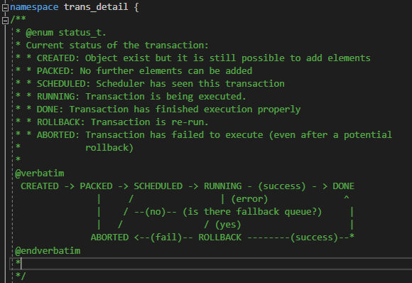
There are several more states represented by the Queue view that describe all of the states a transaction can go through in order to be resolved.
Here is a screenshot of the complete transactions state machine including brief overview of each state:
Now, let's re-visit the vector addition sample again. In this experiment we will try to optimize it by using the full mode of the automated JSON profiler to see the performance impact of our changes.
First we have to set up the profiler:
# in the sdk root
cd build && mkdir config
touch config/sycl_config.txt && echo "enable_profiling = true" >> config/sycl_config.txt
export COMPUTECPP_CONFIGURATION_FILE=config/sycl_config.txt
and set desired output files for the original and optimized versions of the program.
# in the sdk root
cd build && mkdir profiling
touch profiling/vadd_orig.json
export COMPUTECPP_PROFILING_OUTPUT=profiling/vadd_orig.json
Now we only have to compile and run the SYCL vector addition program and the ComputeCpp run-time will generate the file with all the profiling data.
Let's have a look at the visual output by starting with buffer information first:
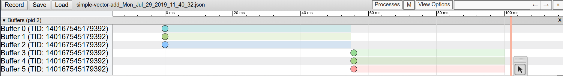
These are all buffer objects for the six vectors we use for the vadd operation - 3 int and 3 float, where 2 of each are input vectors and 1 is the output.
Clicking on the green circle for Buffer 1 allows us to inspect the object that includes information on the time it was created and the arguments that define it, which were explained in the table for Buffer View.
Here is the selection output:
args:   {Count: "8",
         Element Size: "4",
         Range: "(8)",
         Size in Bytes: "32"}
It can be interpreted as follows:
- The buffer object holds an array of eight elements
-
Each element of the array is
4 bytes - The buffer range is with 8 elements in the first dimension
-
The total size of the buffer object is
32 bytes
Additionally, if we were to use the two and three dimensional buffer counterparts, they will be represented almost identically with with the only difference being the range of the elements in the corresponding dimension(s).
2 Dimensional buffer:
args:   {Count: "8",
         Element Size: "4",
         Range: "(2, 4)",
         Size in Bytes: "32"}
3 Dimensional buffer:
args:   {Count: "8",
         Element Size: "4",
         Range: "(2, 2, 2)",
         Size in Bytes: "32"}
Next up is the "Queue" view where we can inspect the performance of the kernel-related commands.
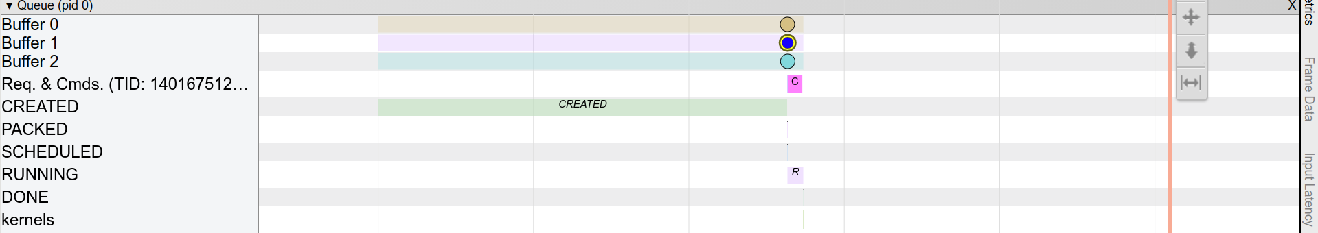
We can also see the access mode and the address space for the buffer (device) data accessors. Clicking on the blue circle for Buffer 1 gives:
args:   {Mode: "Read",
         Space: "Global"}
In order to see how long it takes to enqueue the kernel, we click on the only "COMMAND" in the Req. & Cmds. category, which is shortened to C there. You can zoom in on the tracer window if you wish to focus on a particular item in the trace.
This says that the enqueue took 1.879 ms. Here are the more important details from the selection:
Title             COMMAND
Category          command
Start	          52.766 ms
Wall Duration	  1.879 ms
Args:
    Type          "Enqueue Kernel"
The overall device run-time (submission + kernel execution) can be viewed in the "RUNNING" category by clicking on the purple R there. This shows Wall Duration of 2.041 ms.
Again, here are the important bits of the selection output:
Title             RUNNING
Category          transaction
Start	            52.729 ms
Wall Duration	    2.041 ms
Args:
    Buffer 0      Snapshot of Buffer 0 object @ 52.729 ms
    Buffer 1      Snapshot of Buffer 1 object @ 52.756 ms
    Buffer 2      Snapshot of Buffer 2 object @ 52.761 ms
    kernel        "SYCL_class_SimpleVadd_int_"
The
RUNNING
transaction starts at 52.729 ms while the enqueue kernel command we discussed above was fired at 52.766 ms. This is because of the access acquisition to the data in buffers 0, 1, and 2.
And now let's look at the actual kernel execution time by clicking on the kernel slice in the kernels category. In the image below you can see that the slice is really small but you can select it by using the free selection tool of the tracer.
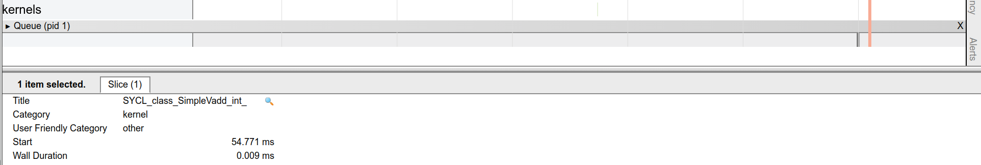
As you can see, you can track every start and duration of a command on the device. The same can be done for Queue (pid 1) which is the second reference of the queue with the SimpleVadd kernel for vectors of type float.
If you are looking for more summarized information of the execution rather than inspecting the timeline, you can make use of another great feature - the "Metadata for Trace" interface. You can click the M button in the top right of the tracer UI and a window that contains information about the Application, the Device it was ran on, the Queue instances and their properties, and Kernel Execution Statistics, will pop out. Here is an example from the same application that we profiled until now.
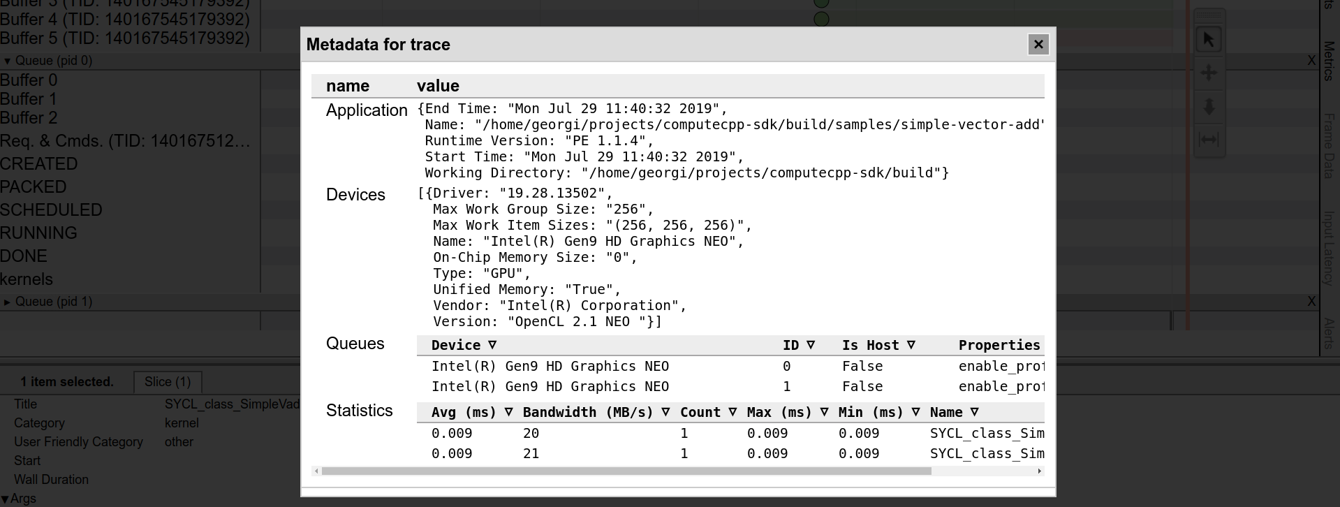
Having profiled the current version of the vector addition kernel, let's attempt an optimization to the vector addition kernel.
First, we need to change the profiling output destination:
# in the sdk build/
export COMPUTECPP_PROFILING_OUTPUT=profiling/vadd_optimized.json
There isn't much that can be done for such a simple kernel, but we can try to do memory coalescing for global memory and run the kernel on a single work-group.
Here is how the kernel code looks like after the modification:
auto kern = [=](cl::sycl::nd_item<1> wi) {
  size_t wiID = wi.get_global_id(0);
  size_t groupSize = wi.get_global_range(0);
  size_t elementsCount = N;
  for (auto i = wiID; i < elementsCount; i += groupSize) {
    accessorC[wiID] = accessorA[wiID] + accessorB[wiID];
  }
};
Briefly, what hopefully happens with this modification is that as each work-item reads its next elements, the reads are combined by the hardware so that we are able to get 64 bytes for each read. This is very specific for the device used to execute this kernel which in this case is an Intel integrated GPU with 64 bytes Global Memory cache line size. This should work equally well for both int and float type elements that are used to test the program.
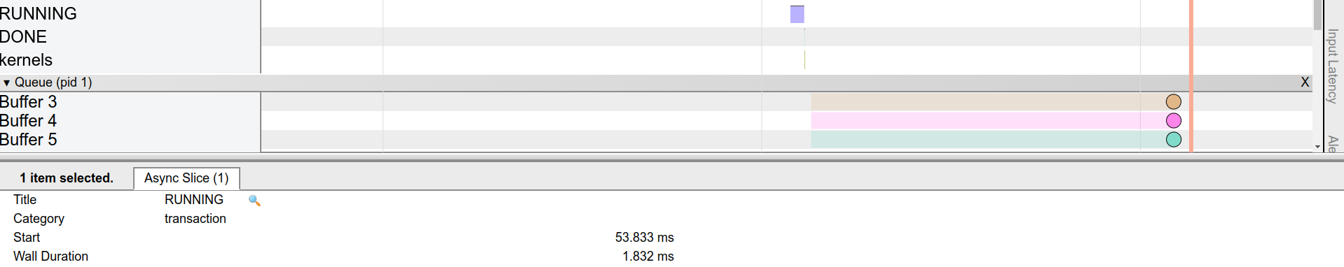
Now let's have a look at the profiling output in the chrome tracer.
The
RUNNING
transaction starts at 1.832 ms as opposed to the 2.041 ms with the non-optimized version.
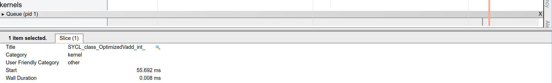
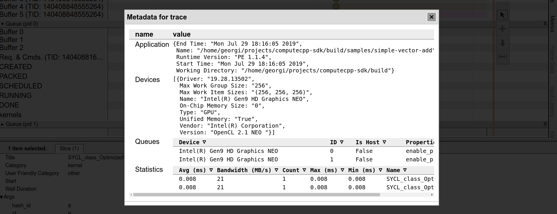
As for the kernel execution time, which was 0.009 ms for both the int and float type kernel instances it is now 0.008 ms.
What is more interesting, however, is that the memory bandwidth is 1mb higher as well - 21 mb in the optimized version versus 20 mb in the original version for int types.
The purpose of this demonstration was not to necessarily optimize the vector addition sample but to demonstrate how handy it is to use the visual representation of the profiling data through the ComputeCpp Professional Edition built-in JSON profiler. It can also benefit the process of optimization when working on SYCL code enabling developers to examine every bit of performance information.
We are adding new features to the profiler, for example, there will be a merging python tool that can merge two profiling output
JSON
files into a single one to better analyze differences in performance and the impact of varying approaches.
You can get in touch to find out more about the ComputeCpp Professional Edition on our developer website.