Alternative machine learning algorithms using SYCL and OpenCL
21 December 2017

Classification is a common use-case for machine learning algorithms and is often achieved using regression. Machine learning (ML) is very computationally intensive so making the most of the available hardware is important to improve the performance of machine learning applications. Heterogeneous computing involves using multiple processor architectures to perform complex operations in parallel and offers a way to improve the performance of machine learning applications. Neural networks have become a well-recognized and widely applied solution to machine learning problems and statistics from Google Books show this upward trend in the last few years.
Using ComputeCpp, the open SYCL standard has been used to enable OpenCL hardware with TensorFlow, a well known deep neural network, but what about techniques that don't use neural networks for machine learning. We will describe several techniques that can be used as an alternative to neural networks. This code was developed as a proof of concept to show what a machine learning application using heterogeneous computing can look like and has been published as an open source project. All of the results in this blog post were computed using an Intel Core I7-6700K CPU and a Radeon R9 Fury Nano GPU with single floating-point precision.
The "SYCL-ML" project and example code is hosted on GitHub.
We developed this project using SYCL and in particular ComputeCpp, which is our implementation of SYCL, to compile and run the code. SYCL is a royalty-free, cross-platform C++ abstraction layer that builds on the underlying concepts, portability and efficiency of OpenCL, while adding the ease-of-use and flexibility of modern C++11/14. SYCL enables single-source development, where the same C++ functions are compiled for both host (typically a CPU) and device (typically a GPU) to construct complex algorithms that use OpenCL acceleration. You can find out more about the SYCL standard on the Khronos website, or dive into the SYCL guide for beginners.
We call this project SYCL-ML and it is a library implementing accelerated versions of four classical machine learning algorithms using the open SYCL standard, these algorithms are:
- Linear Classifier
- Gaussian Classifier
- Gaussian Mixture Model
- Support Vector Machine
Most of the project uses pure SYCL to implement the different kernels however the project has two dependencies that already implement some useful kernels: Eigen and SyclParallelSTL. Eigen is a templated library for linear algebra and Codeplay is working on a custom version that uses SYCL for "Tensor" operations. Eigen is already used in the OpenCL implementation of TensorFlow but SYCL-ML is the proof that Eigen can be used with ease in other simpler SYCL applications. In particular, Eigen is used for its tensor contraction (used as a matrix multiplication) and for some partial reductions (such as summing over a specific dimension of a matrix). The second dependency, SyclParallelSTL, is used to implement some simple kernels in a couple of C++ lines only using the execution policy extension that enables the use of parallel versions of standard C++ methods.
The MNIST dataset
We make use of the MNIST dataset to test each of the classification algorithms presented below. MNIST is a dataset composed of labelled examples of handwritten digits, and is commonly used as a benchmark for classification algorithms. The images are 28 by 28 pixels in grayscale and the labels are the 10 digits.
Because the algorithms are not specific to images an "image" will be mentioned as an "observation". For MNIST the size of an observation is 28*28=784, there are 60,000 observations in the training set and 10,000 in the test set.
The frequency of each label is about the same in both the training set and test set, for this reason the results will only show the success rate (precision and recall are roughly the same).
Implemented algorithms
Principal Component Analysis
PCA is an unsupervised algorithm that finds a new basis for any given dataset in order to reduce the dimensionality of the observations to any chosen integer N. It can be proven that in order to lose as little information as possible, the optimal basis should be a set of N eigenvectors of the covariance matrix. The eigenvalue corresponding to an eigenvector represents the "amount of information" this vector holds. Thus choosing the N eigenvectors with the largest eigenvalue gives you the optimal basis. A new dataset can then be created in this basis, effectively reducing the size of each observation to N.
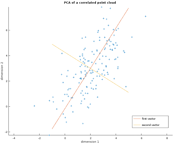
The image below shows a random point cloud of 150 two-dimensional observations where the two dimensions are correlated. The two vectors in red and orange are the output of the PCA i.e. the basis we could use to transform this dataset. It shows that the first one (in red) is more important as the points are more spread out along this axis.
The more correlated the data is, the fewer vectors are actually needed. In particular for MNIST, 86.2% of the information is kept with only 64 eigenvectors and 93.6% with 128. This was to be expected since a lot of the pixels in the corner are the same across the observations. Besides, the information dropped most of the time is noise that does not help the classification because it will be shown with the Gaussian classifier and the Gaussian Mixture Model.
So applying the PCA before a classifier allows us to reduce both memory consumption (each observation is smaller) and execution time (every operation on the dataset itself will be faster). It is also a way to control the size of an observation without padding the data with zeros. In particular, the observation's size of some of the following implementations must be a power of two.
The current implementation relies on the SVD decomposition to compute the eigenpairs based on this paper. This function has not been optimized yet.
The helper class apply_pca makes it nice and easy to use. The example below is extracted from example/src/mnist/run_classifier.hpp which will be explained in more detail later. Note that the same base must be used to transform the train and test data which is why the eigenvectors are computed only when compute_and_apply is called. The argument keep_percent sets the minimum "amount of information" we have to keep using the new basis. It is a percentage in [0, 1] where zero will disable the PCA and one will keep all the basis vectors. The argument min_nb_vecs lets the user choose a specific minimum number of basis vector to use (useful to have a power of two). The number of eigenvectors will be chosen so that both constraints are respected.
ml::pca_args pca_args;
pca_args.keep_percent = 0.8;
pca_args.min_nb_vecs = 64;
auto sycl_train_data = apply_pca.compute_and_apply(q, sycl_train_data_raw, pca_args);
auto sycl_test_data = apply_pca.apply(q, sycl_test_data_raw);
Linear Classifier
The linear classifier is one of the simplest supervised classification algorithms. As the name suggests, it should only be used when the data is linearly separable. Formally a linear classifier can be seen as a naive Bayes classifier with a Gaussian distribution assuming the covariance matrices are identities.
As with many machine learning classification algorithms, the algorithm consists of separate training and classification or inference stages.
The training stage consists of computing an average observation for each unique label in the classification set. Given a new observation, the inference step selects the label with the smallest Euclidean distance between our new observation and the learned average observations.
In terms of operations that can be accelerated on the device, the training step has as many partial reductions as there are labels. Each reduction is a sum over the number of observations of the current label. The inference has one partial reduction over the size of observation to compute the distance and another on the number of labels to select the minimum distance. The rest are element-wise operations which are easily accelerated on the device as well.
These two images show a dataset in two dimensions with two labels (blue and green). The left one shows the learned average for each label as a small circle. The bigger circle represents the points where the distance is the same for both labels. One way to think about these circles is to picture them growing progressively larger until they collide and create a line called the separator. This visualization will help us to understand the Gaussian classifier. The right image shows the separator.
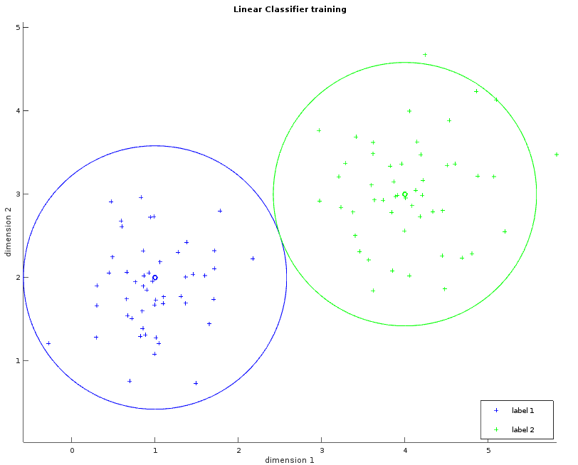
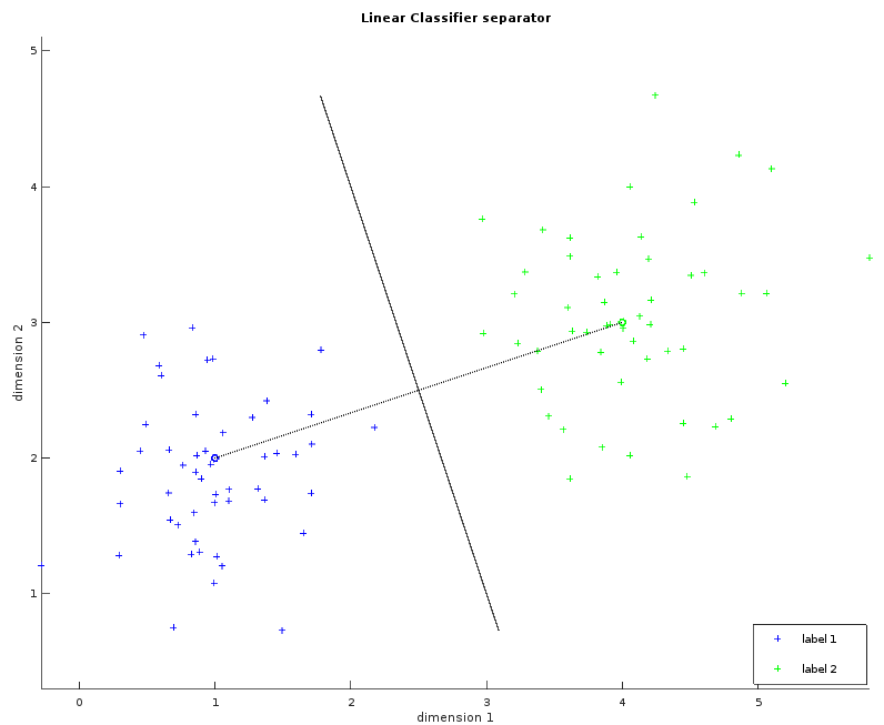
Whilst the examples above only illustrate a simple example consisting of two fact dimensions, two labels and a single separating plane, the algorithm can be easily generalized with more dimensions and more labels. The observations within the MNIST dataset violate our requirement that the data be linearly separable. Despite this, the linear classifier can still be applied in order to provide our first result, albeit with reduced classification accuracy.
The linear classifier can be run on MNIST using example/src/mnist/run_lin_classifier.cpp and this is the line where the classification is executed:
run_classifier<ml::linear_classifier<ml::buffer_data_type, uint8_t>>(mnist_path, pca_args);The results are given below. It is possible to see that reducing the size of an observation of a factor close to 10 speeds up the training time by a factor 2 and the inference time by a factor 10 at the cost of a slightly worse success rate. All things considered, the success rate is rather good given the time spent in training and inference, but there is definitely some room for improvement.
| Observation size | Training rate (obs/s) | Inference rate (obs/s) | Success rate (%) | |
|---|---|---|---|---|
| MNIST (raw) | 784 | 4.754E5 | 1.241E5 | 82.03 |
| MNIST (pca) | 128 | 9.927E5 | 9.952E5
| 81.98 |
| MNIST (pca) | 64 | 9.930E6 | 1.882E6 | 81.81 |
Gaussian Classifier
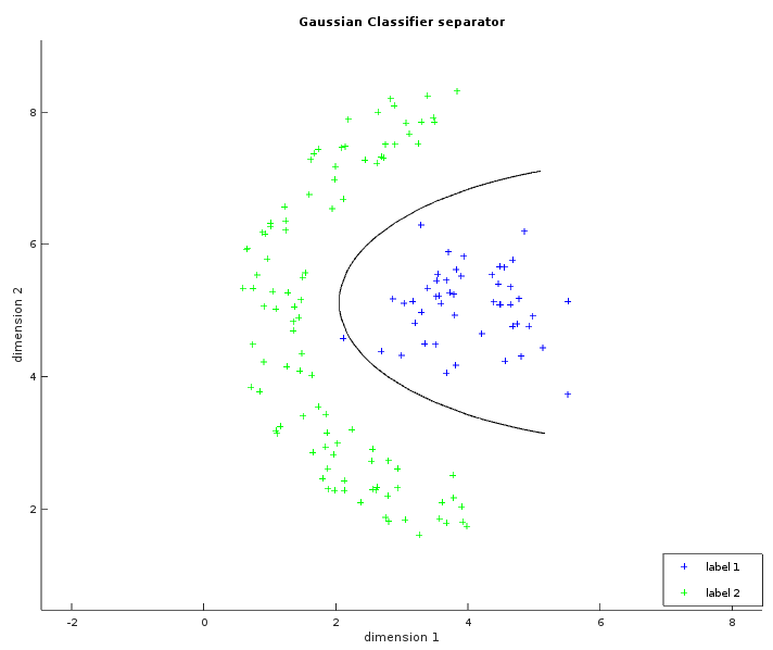
The Gaussian classifier is a more generalized version of the linear one. We now assume that the data are normally distributed according to their class. This will allow an hyperbolic separator enabling us to solve many more different kinds of problems.
On top of the average observation, the classifier also needs to learn the covariance matrix of each label. One way to interpret this is to think of this matrix as a way to tell which variables (or pixels for MNIST) are important and which are not for a specific label. The covariance matrix is then used during inference to compute the Mahalanobis distance instead of the Euclidean one. This distance is actually the part inside the exponential of the Gaussian Multivariate formula.
Note that the use of PCA is required to remove the useless variables, i.e. the variables that have a variance of zero. The reason for this is that the covariance matrix needs to be inverted.
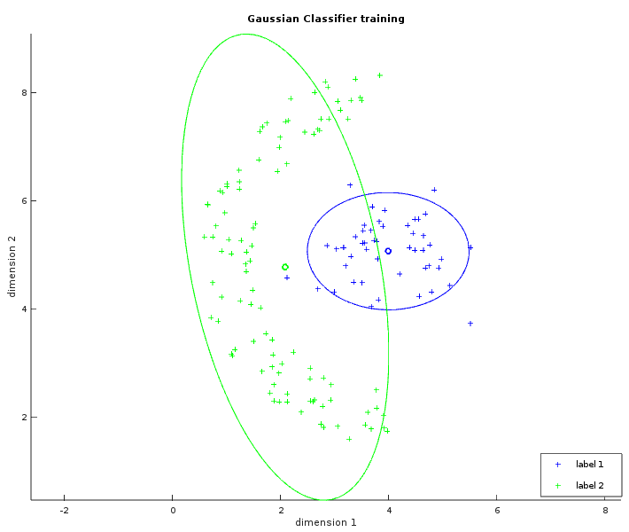
The two images below show some labelled data that is not linearly separable. The left image is similar to what has been shown with the linear classifier. The ellipses in green and blue were created from a circle with the same radius transformed by their respective covariance matrix (and centered on their respective average). In the whitened space of the first label, each point of the blue ellipse is at the same distance to the blue center. This distance is also the same in the whitened space of the second label between each point of the green ellipse and the green center. The right image shows the learned separator which is the set of points with the same likelihood to be either labels. The result is not perfect but is still better than what a linear classifier could do.
Now the actual implementation does not use the covariance matrix for performance and precision issues. The Mahalanobis distance is usually written:
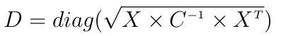
where X is some centered data (each observation is a row), C is some covariance matrix and diag extracts the diagonal of the given matrix.
This is costly because of the inversion of the full matrix C and the two matrix multiplications. Another way to write this is:
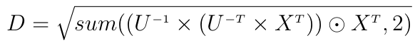
where U is the upper Cholesky decomposition of C, "odot" is the element-wise multiplication and sum is a partial sum here reducing the second dimension.
This is faster because U is an upper triangular matrix and each inversion followed by a product can be done in a single step by a triangular solver. However computing the Cholesky decomposition is not numerically stable and can fail because of the rounding errors introduced by the floating-point representation. The trick is to instead compute the QR decomposition of the dataset. For some dataset A with N observations one has:
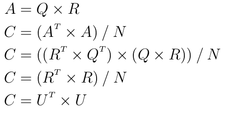
because Q is orthogonal. Hence:
assuming all diagonal values of R were chosen to be positive.
This last simple equation means that it is possible to use the nicer formula of the Mahalanobis distance without actually computing the covariance matrix and the inefficient Cholesky decomposition but with a QR decomposition instead.
Also note that the log of the Gaussian distribution has to be used to keep values in a reasonable range.
To put it in a nutshell, rewriting the distance formula to use the QR decomposition instead of the covariance matrix speeds up the inference time a lot at a reasonable cost during the training time.
During the training, the QR decomposition is the most expensive operation. SYCL-ML uses a version of the Householder QR algorithm that computes only the R matrix. Each row of the R matrix is computed iteratively and each row depends on the result of the previous one, so for this reason the performances on the device are not optimal. A blocked version of this algorithm exists but hasn't been implemented yet.
The inference time is bounded by the triangular solver. Once again each row of the output depends on the result of the previous row which makes the algorithm difficult to optimize on a device.
The Gaussian classifier is run with the following code in example/src/mnist/run_gauss_classifier.cpp:
using distribution_t = ml::buffered_log_gaussian_distribution<ml::buffer_data_type>;
run_classifier<ml::bayes_classifier<distribution_t, uint8_t>>(mnist_path, pca_args);
Below are the results of a Gaussian classifier with MNIST. It may look surprising that the success rate is better with 64 variables even though more information is lost than with 128. The reason is that the information lost appeared to be non relevant for the classification however this is not always true.
|
|
Observation size | Training rate (obs/s) | Inference rate (obs/s) | Success rate (%) |
|---|---|---|---|---|
| MNIST (pca) | 128 |
3.356E4
|
3.477E4
|
95.46 |
| MNIST (pca) | 64 | 8.171E4 | 8.827E4 | 96.14 |
Gaussian Mixture Model
The Gaussian Mixture Model (GMM) is an improvement on the previously seen Gaussian classifier. The idea is that a single Gaussian distribution may not always be enough to grasp the shape of the data with the same label. Rather than trying to fit a more complex distribution to capture this complexity, it is possible to fit multiple Gaussian distributions. The number of distributions to fit is defined by the parameter M so the total number of distributions is now M times the number of labels.
The difficult part is that the distributions of a same label should not merge in the same distribution. The Expectation Maximization (EM) algorithm makes sure that this does not happen. The EM iteratively maximizes the likelihood of each distribution. It partitions the data in M subsets that are used in the next iteration to compute the new parameters of each distribution (here the average and the covariance matrix). The algorithm stops when the likelihood is stable enough meaning that the distributions don't move much. Note that any distribution can be used, the Gaussian being the most common one.
The current implementation initializes the first parameters for the first iteration randomly. Using clustering techniques to compute the first parameters would ensure a faster convergence but this has not been implemented yet. The implementation also uses the log version of the classical EM to keep values in a reasonable range.
The operations specific to the EM algorithm are either element-wise operations or partial reductions (computing a sum or finding a maximum over the rows). These are pretty well optimized in the current implementation, however the distance of the given distribution needs to be computed during the training as well which now makes the triangular solver the most expensive operation during the training. This inference time is still bounded by the triangular solver as well.
The image below shows the result of the GMM training in a similar way to the Gaussian classifier. Here M=4 meaning that the GMM is trying to fit four Gaussians for each label. The separator would be harder to draw in the general case because it can be multiple hyperbolic functions, here it is easy to guess what it would look like.

The GMM is run with example/src/mnist/run_gmm.cpp:
using data_t = ml::buffer_data_type;
using label_t = uint8_t;
using distribution_t = ml::buffered_log_gaussian_distribution<data_t>;
using model_t = ml::log_model_per_label<M, distribution_t>;
static constexpr unsigned M = 8;
run_classifier<ml::em_classifier<label_t, model_t>>(mnist_path, pca_args);
Without any surprises, fitting more distributions gives a better success rate but a slower classifier.
|
|
Observation size | M |
Training rate (obs/s) | Inference rate (obs/s) | Success rate (%) |
|---|---|---|---|---|---|
| MNIST (pca) | 64 | 2 |
1.604E3
|
4.281E4
|
96.54 |
| MNIST (pca) | 64 | 8 | 4.456E2 | 1.145E4 | 97.41 |
Support Vector Machine
Support Vector Machines (SVM) provide a completely different approach from those presented so far. The main idea behind it is to cleverly select samples that are close to the theoretical separator. These samples are the support vectors (SVs) and will define the margin i.e. the area between the SVs of the first label and the SVs of the second label. The separator will be in the middle of the margin and the most generic separator will be found by maximizing the margin. This Wikipedia page explains more detail on how SVMs work very well.
The implemented SVM is a C-SVM which allows us to use both soft-margin and hard-margin SVMs depending on the C parameter. A hard-margin SVM (with C "big enough") forbids us to mis-classify a training example. This also means that the SVM cannot converge if the data is not separable with the given kernel. The smaller C is the softer the SVM becomes and the more mis-classification is allowed. This can be useful as the training set is often noisy.
The implementation is very similar to that found in libSVM, both of which are based on this paper. The main difference as a user is that SYCL-ML does not sort the data per label when there are only two labels whereas libSVM does. This will give different results when the dataset has exactly two labels. It uses the One vs One method to combine multiple binary SVMs into one multi-class classifier. This method usually gives better results than One vs All.
In general, SVMs are difficult to parallelize; some more work can definitely be done in this area.
One of the challenges other than parallelization is how to cache the kernel matrix efficiently. The easiest solution is to compute it once and store it, but this is usually not possible because of the limit on the buffer size. The solution is to cache only a fixed number of rows even if it means recomputing some of the rows. By default, a maximum of two rows are cached, it is also possible to ask for the whole matrix to be cached.
The user can define their own kernel to use but the four most common ones are already available:
- Linear: u * v'
- Polynomial: (g .* (u * v') .+ c) .^ d
- RBF: exp(-g .* |u - v|^2)
- Sigmoid: tanh(g .* (u * v') .+ c)
The SVM is run on MNIST using the code in example/src/mnist/run_svm.cpp. The argument nb_cache_line is usually set to 2 meaning that 2 rows of the kernel matrix are cached.
using data_t = ml::buffer_data_type;
using label_t = uint8_t;
using svm_kernel_t = ml::svm_rbf_kernel<data_t>;
using svm_type_t = ml::svm<svm_kernel_t, label_t>;

const data_t C = 5;
const svm_kernel_t ker(gamma);
run_classifier(mnist_path, pca_args, svm_type_t(C, ker, nb_cache_line, tol));
The table below shows the results for several configurations of the SYCL-ML SVMs. While it is possible to use the SVM without a PCA, it is definitely slower and less accurate to use the raw data. The SVM with a polynomial kernel already gives some good results for a high training rate and inference rate. After some fine tuning, the RBF kernel turns out to be the most adapted. The reason the inference rate is lower for RBF kernels is that more SVs are selected.
|
|
Observation size | Kernel | SVM parameters |
Training rate (obs/s) |
Inference rate (obs/s) |
Success rate (%) |
|---|---|---|---|---|---|---|
| MNIST (raw) | 784 | Polynomial d=2 g=1 c=1 | C=1000 tol=0.01 | 1.445E2 | 6.790E3 | 98.10 |
| MNIST (pca) | 64 | Polynomial d=2 g=1 c=1 | C=1000 tol=0.01 | 2.038E2 | 3.775E4 | 98.30 |
| MNIST (raw) | 784 | RBF gamma=0.05 | C=5 tol=0.01 | 4.305E0 | 8.887E0 | 98.37 |
| MNIST (pca) | 64 | RBF gamma=0.05 | C=5 tol=0.01 | 2.100E2 | 2.495E2 | 98.66 |
| MNIST (pca) | 64 | RBF gamma=0.05 | C=5 tol=0.1 | 3.926E2 | 2.983E2 | 98.66 |
Usage example
All the examples of the classifiers use the example/src/mnist/run_classifier.hpp function which will be explained now. The usage of the SYCL API is non-intrusive meaning that very little SYCL specific code is actually visible here.
First let's start with the prototype and some setup.
template <class ClassifierT>
void run_classifier(const std::string& mnist_path,
                    const ml::pca_args<typename ClassifierT::DataType>& pca_args,
                    ClassifierT classifier = ClassifierT()) {
  // The TIME macro creates an object that will print the time elapsed between its
  // construction and destruction
  TIME(run_classifier);

  using DataType = typename ClassifierT::DataType;
  using LabelType = typename ClassifierT::LabelType;

  // MNIST specific
  std::vector<LabelType> label_set(10);
  // Create the set of labels here instead of computing it during the training
  std::iota(label_set.begin(), label_set.end(), 0);
  const DataType normalize_factor = 255;  // Data will be shifted in the range [0, 1]

  // Load and save options
  const bool load_classifier = false;
  const bool save_classifier = false;

  // What the classifier will compute
  std::unique_ptr<LabelType[]> host_predicted_test_labels;
Next is the first bit of code related to SYCL, the creation of the queue. In SYCL, the queue is tied to a single OpenCL accelerator device and context. The queue allows us to submit kernels for execution on the accelerator, so most functions will require access to it.
Creating the queue is usually as simple as calling the default constructor and the SYCL runtime will automatically select the first suitable accelerator for us. Here this is handled by the create_queue function because a few additional steps are required:
- Query some device constants for later use
- Initialize Eigen and get the SYCL queue that has been created
- Launch a first empty kernel to avoid measuring the OpenCL overhead during the training
A scope is opened before creating the queue in order to better control when to destroy it. The destruction of the queue will also release the OpenCL context.
{ // Scope with a SYCL queue
  cl::sycl::queue& q = create_queue();
The helper class for the PCA will also be used.
ml::apply_pca<DataType> apply_pca;Next the data will be loaded on the host and copied on the device. The ml::matrix_t and ml::vector_t classes are wrappers around the cl::sycl::buffer class for 1D buffer. These wrappers hold a data_range and a kernel_range, the kernel_range can be a larger range than the data_range for better performance (usually the next power of two). When one of these buffers is created with a host pointer, the data will be copied to the device.
Another scope is opened to destroy any buffers used for the training only. Notice that the training data will not be transposed, the observation size will be padded to a power of two and the data will be normalized in the range [0, 1]. The resulting matrix will be of size nb_train_obs * padded_obs_size in the row major layout.
The call to compute_and_apply will only compute the PCA if this is the first time running it with this number of basis vectors, otherwise it will be loaded from the disk.
{
  unsigned obs_size, padded_obs_size, nb_train_obs;
  // Load tain data
  ml::matrix_t<DataType> sycl_train_data;
  {
    std::shared_ptr<DataType> host_train_data =
      read_mnist_images<DataType>(mnist_get_train_images_path(mnist_path), obs_size,
                                  padded_obs_size, nb_train_obs, false, true,
                                  normalize_factor);
    ml::matrix_t<DataType> sycl_train_data_raw(std::move(host_train_data),
                                               cl::sycl::range<2>(nb_train_obs,
                                                 padded_obs_size));
    sycl_train_data_raw.data_range[1] = obs_size;  // Specify the real size of an observation
    sycl_train_data_raw.set_final_data(nullptr);

    sycl_train_data = apply_pca.compute_and_apply(q, sycl_train_data_raw, pca_args);
  }

  // Load labels
  std::shared_ptr<LabelType> host_train_labels =
    read_mnist_labels<LabelType>(mnist_get_train_labels_path(mnist_path), nb_train_obs);
  ml::vector_t<LabelType> sycl_train_labels(std::move(host_train_labels),
                                            cl::sycl::range<1>(nb_train_obs));
  sycl_train_labels.set_final_data(nullptr);
The classifier can then start its training. It could also save the training result to the disk or load a previous training from the disk but this is omitted here for clarity.
{
    TIME(train_classifier);
    classifier.set_label_set(label_set);  // Give the sets of labels to avoid computing them during the training
    classifier.train(q, sycl_train_data, sycl_train_labels);
    q.wait(); // wait to measure the correct training time
  }
} // End of train
In a very similar way, the classifier can then be used to predict the labels of the test data:
{
  unsigned obs_size, padded_obs_size, nb_test_obs;
  ml::matrix_t<DataType> sycl_test_data;
  { // Load test data
    std::shared_ptr<DataType> host_test_data =
      read_mnist_images<DataType>(mnist_get_test_images_path(mnist_path), obs_size,
                                  padded_obs_size, nb_test_obs,
                                  false, true, normalize_factor);
    ml::matrix_t<DataType> sycl_test_data_raw(host_test_data,
                                              cl::sycl::range<2>(nb_test_obs,
                                                padded_obs_size));
    sycl_test_data_raw.data_range[1] = obs_size;  // Specify the real size of an observation
    sycl_test_data_raw.set_final_data(nullptr);

    sycl_test_data = apply_pca.apply(q, sycl_test_data_raw);
  }

  { // Inference
    TIME(predict_classifier);
    ml::vector_t<LabelType> sycl_predicted_test_labels = classifier.predict(q, sycl_test_data);
    // Can be round up to a power of 2
    auto nb_labels_predicted = sycl_predicted_test_labels.get_count();
    host_predicted_test_labels =
      std::unique_ptr<LabelType[]>(new LabelType[nb_labels_predicted]);
    sycl_predicted_test_labels.set_final_data(host_predicted_test_labels.get());
    q.wait(); // wait to measure the correct prediction time
  }
} // End of tests
Now SYCL is not needed anymore, the context can be cleared. Closing the scope is usually enough to clear everything, here clear_eigen_device is also needed to release a singleton.
  clear_eigen_device();
} // SYCL queue is destroyed
Finally we can evaluate the classifier's prediction and end the function:
  unsigned nb_test_obs;
  std::shared_ptr<LabelType> host_expected_test_labels =
    read_mnist_labels<LabelType>(mnist_get_test_labels_path(mnist_path), nb_test_obs);
  classifier.print_score(host_predicted_test_labels.get(), host_expected_test_labels.get(),
                         nb_test_obs);
}
So that's everything for the run_classifier function. The important lines in this function that actually submit kernels are the calls to:
- compute_and_apply and apply for the preprocessing step
- train and predict for the classifying step.
To have a better idea of what the code looks like inside these functions, let's have a look at a common function used for all inplace binary operations on matrices.
As mentioned before, matrix_t is a wrapper around a cl::sycl::buffer of 1 dimension and we can see two advantages of this wrapper here:
- the SYCL-ML API forces you to use matrices when it is suited, in particular transposing with D1 and D2 only makes sense for matrices. It is still possible to use the matrix as a simple 1D buffer.
- the global and local range sizes to use for the kernel is given by the matrix itself with get_nd_range and is not needed as an additional parameter. The local range is computed once on matrix creation depending on device parameters.
Finally, each kernel must have a unique name given at compilation time as a template parameter. Here it is NameGen<0, ml_mat_inplace_binary_op<D1, D2>, T, BinaryOp>. It is important that all template parameters of a function appear in the kernel name otherwise calling the function with different template parameters can lead to the same kernel name.
template <data_dim, data_dim>
class ml_mat_inplace_binary_op;

template <data_dim D1 = LIN, data_dim D2 = LIN, class T, class BinaryOp>
void mat_inplace_binary_op(queue& q, matrix_t<T>& in_out1, matrix_t<T>& in2,
                           BinaryOp op = BinaryOp()) {
  // Check that the number of rows are the same
  assert_eq(access_ker_dim<D1>(in_out1, 0), access_ker_dim<D2>(in2, 0));
  // Check that the number of columns are the same
  assert_eq(access_ker_dim<D1>(in_out1, 1), access_ker_dim<D2>(in2, 1));

  q.submit([&](handler& cgh) {
    // accessor will be transposed if D1=TR
    auto in_out1_acc = in_out1.template get_access_2d<access::mode::read_write, D1>(cgh);
    // accessor will be transposed if D2=TR
    auto in2_acc = in2.template get_access_2d<access::mode::read, D2>(cgh);
    using kernel_name_t = NameGen<0, ml_mat_inplace_binary_op<D1, D2>, T, BinaryOp>;
    cgh.parallel_for<kernel_name_t>(in_out1.template get_nd_range<D1>(),
                                    [=](nd_item<2> item) {
      auto row = item.get_global(0);
      auto col = item.get_global(1);
      in_out1_acc(row, col) = op(in_out1_acc(row, col), in2_acc(row, col)); // Apply op
    });
  });
}
Conclusion
To summarize, we have seen four different ways of classifying data with each method more complex than the previous. As with neural networks, they are well suited for classification and regression, although they usually perform worse on complex image classification. The use of SYCL enabled us to write the whole library in modern C++14 with all of the computationally intensive operations accelerated on a device that would not have been possible any other way.
If you want to run the data classification yourself you'll find instructions in the README file, and because this uses SYCL they can be executed on any hardware that supports OpenCL SPIR instructions. Feel free to send in any improvements you make to the GitHub repository and raise any issues through the tracker.